Pipeline Parallelism(PP)
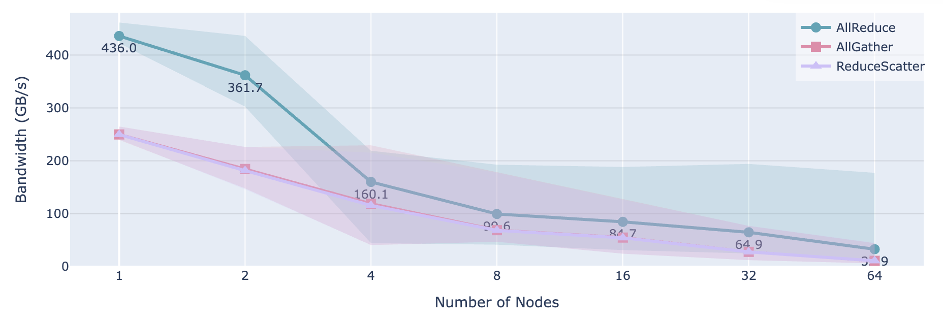
回顾TP当中,我们将tensor并行性的规模超过一个node上的4或者8个gpu的时候会迫使我们用低带宽lower-bandwidth的网络通讯,简言之走了net(机间的IB,roce等)。
sequence和context的并行对处理长序列输入有帮助,但是model本身参数太大的话这两种并行就没有什么用了。对于超过70B+ parameters的model,光是werights就会超过4-8个gpu的显存。这就需要用流水线并行pipeline parallelism来处理,就是将模型的计算层拆分成好几段,每个gpu分一些计算层,然后从前往后依次传递计算,从而避免了每个gpu必须加载完整的模型。
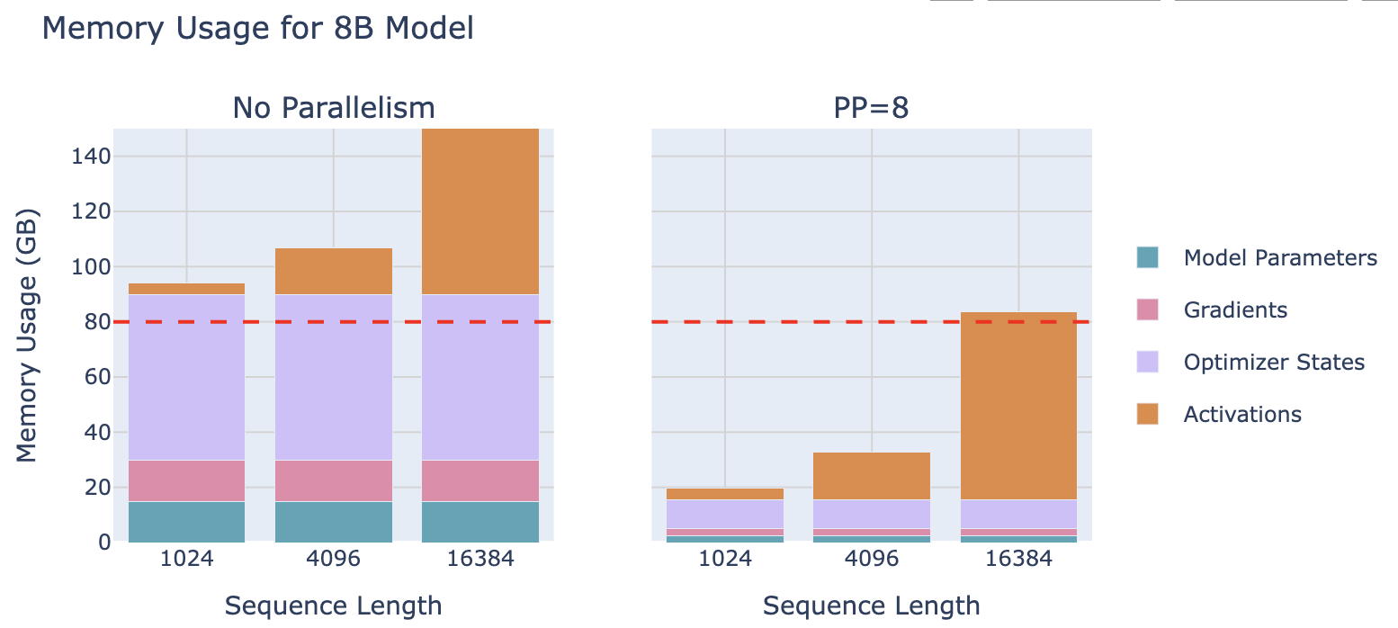
上图中可以看到模型参数被均分了,但是每个gpu上占用的Activations激活值并没有减少!所以PP不会降低激活值的显存使用
原因:模型训练的时候反向传播得等前向传播结束。那么,使用PP的时候每个GPU就必须完成PP个前向传播。PP中会将一个完整的batch切成多个小的micro-batches,每个GPU轮流处理这些micro-batches,然后整个流水线才能开始反向传播。那么backward前,每个GPU处理了1/PP的网络层(PP个micro-batches),每个micro-batches产生自己的激活值是activs / pp, 内存需求就是。结论:激活值占用的总内存和不用PP流水线并行差不多。
这就引入了新的通信模式,在ZeRO-3(数据并行的优化方法)中我们的重点是多GPU之间同步参数和梯度,而这里PP的核心就变成了:传递前向传播中产生的激活值tensors。要高效实现起来很难,面临同步,显存压力和通信带宽等挑战。
1. Splitting layers on various nodes - All forward, all backward 模型层分到多个节点上-整体前向和反向
这里从简单的PP逻辑开始,然后引出潜在的问题。
首先,各个layer分配到多个GPU上,例如GPU1处理模型前几层,GPU002处理模型中间几层,以此类推。这样就可以吧一个batch的数据按顺序传递给每个GPU,模型的不同部分一次执行。
此时会face第一个问题:机间的带宽会很低,因为我们只send了model深度的位置的中等大小激活值一次(GPU001到GPU002),与TP(每一层就多次通信)截然不同。这里的逻辑是顺序的依次的执行,在并行世界并不高效。现在的训练都讲究一个computation and communication overlap来提升效率,这个PP显得有点落后。
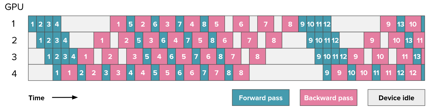
如果绕过本质上的“顺序行”就可以让GPU始终繁忙。做最naive的forward和backward的时候GPU利用率如下:
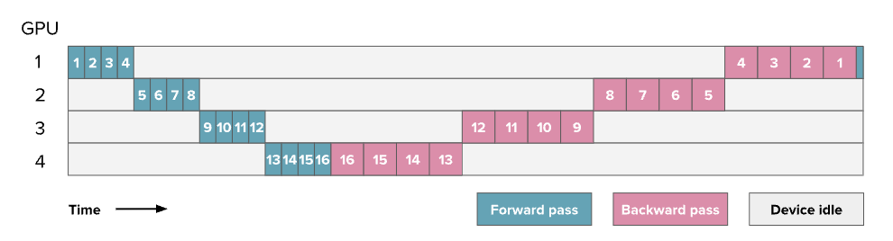
这里灰色部分表示剩余的空闲时间,也叫气泡(bubble)。现在假设t_f是前向传播时间,t_b是反向传播时间。并假设反向传播时间是前向传播时间的2倍。理想情况下完美的PP耗时应该是:t_id = t_f + t_b。实际中由于bubble会产生额外的时间损失t_pb = (p - 1) x (t_f + t _b),这里p是并行度即GPU数量。可以用以下公式计算“气泡时间”相对于“理想总时间”的比例:
r_bubble = ((p − 1) × (t_f + t_b)) / (t_f + t_b) = p − 1即两卡的话bubble开销是1倍,8卡的话就是7倍。实验的时候随着PP阶段数的增加,bubble会变的更大导致GPU利用率下降。所以PP就要更聪明的调度:
现在将一个batch变为一堆micro-batches,使他们能够parallel的处理,下图为8个micro-batches
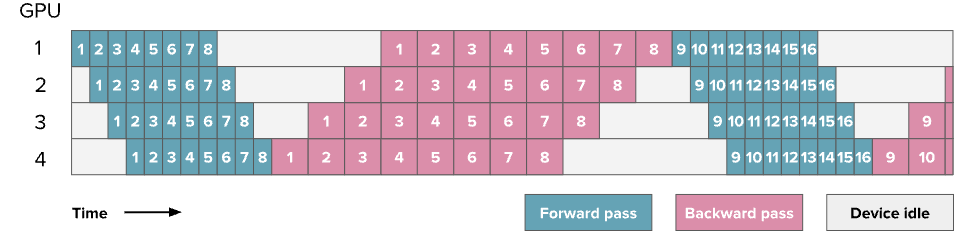
图中展示的调度方式被称为 全前向、全反向(AFAB,All Forward, All Backward) 调度,因为我们先完成所有的前向传播步骤,然后再统一执行所有的反向传播步骤。这种方式的优势在于:前向与反向步骤仍然是整体上顺序执行的,因此我们得以保留我们原本训练代码的整体结构与逻辑。但是这是最简单最容易实现的流水线。Picotron中有AFAB的完整实现如下:
def train_step_pipeline_afab(model, data_loader, tensor_shapes, device, dtype):
    logging_loss: torch.float32 = 0.0
    input_tensors, output_tensors = [], []
    requires_grad_sync = pgm.process_group_manager.cp_dp_world_size > 1

    for _ in range(data_loader.grad_acc_steps): # All forward passes
        input_tensor = pipeline_communicate(operation='recv_forward', shapes=tensor_shapes, device=device, dtype=dtype)
        batch = next(data_loader)
        batch["hidden_states"] = input_tensor.to(device) if input_tensor is not None else input_tensor
        output_tensor = model.forward(input_ids=batch["input_ids"].to(device), position_ids=batch["position_ids"].to(device), hidden_states=batch["hidden_states"])
        pipeline_communicate(operation='send_forward', tensor=output_tensor, device=device, dtype=dtype)

        # calculate loss on the last stage
        if pgm.process_group_manager.pp_is_last_stage:
            output_tensor = F.cross_entropy(output_tensor.transpose(1, 2), batch["target_ids"].to(device), reduction='mean')
            logging_loss += output_tensor.item() / data_loader.grad_acc_steps

        input_tensors.append(input_tensor)
        output_tensors.append(output_tensor)

    for ith_microbatch in range(data_loader.grad_acc_steps): # All backward passes
        if requires_grad_sync:
            is_last_iteration = (ith_microbatch == data_loader.grad_acc_steps - 1)
            model.require_backward_grad_sync = is_last_iteration
        output_tensor_grad = pipeline_communicate(operation='recv_backward', shapes=tensor_shapes, device=device, dtype=dtype)
        input_tensor, output_tensor = input_tensors.pop(0), output_tensors.pop(0)
        input_tensor_grad = model.backward(input_tensor, output_tensor, output_tensor_grad)
        pipeline_communicate(operation='send_backward', tensor=input_tensor_grad, device=device, dtype=dtype)

    return logging_loss
现在估算一下这里bubble的情况,现在要处理 m 个 micro-batches,理想的总时间是:t_id = m × (t_f + t_b),气泡占比可表示为:
也就是说:如果8个GPU 2个micro-batches的话 气泡占比就是7 / 2 = 350%,如果增加micro-batches为8的话气泡占比就是7 / 8 = 87.5%。
正如我们所见,我们可以通过增加 micro-batches 的数量,来抵消一部分流水线阶段的低效,将气泡的尺寸减少。
然而,会随之带来第二个问题就是在反响传播前这里所有的micro-batches都要保留激活值,这会很容易导致内存爆炸(memory explosion)。所以我们可以尝试在前向传播尚未完全结束的时候就开始执行反向传播,在不影响计算的前提下,尽早释放一些激活值的内存占用。于是1F1B诞生:
2. One Forward, One Backward and Llama 3.1 schemes一次前向一次后向(1F1B)和llama 3.1调度方案
核心思想:尽早开始反向传播,这种叫1F1B。因为中间的稳定阶段会出现交替的forward和backward。
对比AFAB的图,bubble并没有降低,训练效率本身没有提升。但是现在1F1B同时最多只需要为p个micro-batches(p 是流水线并行度,即 GPU 数)保存激活值,而不是像 AFAB 调度中那样需要为 m 个 micro-batches(即整个批次数量)保存激活值。此时再增加更多的micro-batches就可以降低气泡的大小。
1F1B调度的主要复杂性现在就是forward和backward不是顺序执行,而是在不同device上交错并行的执行。这正是为什么实现流水线并行通常需要对训练代码和模型代码进行较大改动的原因。这也是为什么像 Hugging Face 的 Picotron、DeepSpeed 的 PipeDream 等工具出现的重要原因,它们来封装这套复杂调度,而不是再用pytorch默认的训练逻辑。下面是1F1B代码:
1F1B PP implementation in Picotron
def train_step_pipeline_1f1b(model, data_loader, tensor_shapes, device, dtype):
    num_warmup_microbatches = min(pgm.process_group_manager.pp_world_size - pgm.process_group_manager.pp_rank - 1, data_loader.grad_acc_steps)
    num_microbatches_remaining = data_loader.grad_acc_steps - num_warmup_microbatches
    logging_loss, input_tensors, output_tensors  = 0.0, [], []
    requires_grad_sync = pgm.process_group_manager.cp_dp_world_size > 1

    def _forward_step(input_tensor):
        batch = next(data_loader)
        batch["hidden_states"] = input_tensor.to(device) if input_tensor is not None else input_tensor
        output_tensor = model.forward(input_ids=batch["input_ids"].to(device), position_ids=batch["position_ids"].to(device), hidden_states=batch["hidden_states"])

        # calculate loss on the last stage
        if pgm.process_group_manager.pp_is_last_stage:
            output_tensor = F.cross_entropy(output_tensor.transpose(1, 2), batch["target_ids"].to(device), reduction='mean')
            nonlocal logging_loss
            logging_loss += output_tensor.item() / data_loader.grad_acc_steps
        return output_tensor

    for _ in range(num_warmup_microbatches): # Warmup forward passes
        input_tensor = pipeline_communicate(operation='recv_forward', shapes=tensor_shapes, device=device, dtype=dtype)
        output_tensor = _forward_step(input_tensor)
        pipeline_communicate(operation='send_forward', tensor=output_tensor, device=device, dtype=dtype)
        input_tensors.append(input_tensor)
        output_tensors.append(output_tensor)

    if num_microbatches_remaining > 0:
        input_tensor = pipeline_communicate(operation='recv_forward', shapes=tensor_shapes, device=device, dtype=dtype)

    if requires_grad_sync:
        model.require_backward_grad_sync = False

    for ith_microbatch in range(num_microbatches_remaining):  # 1F1B steady state
        is_last_iteration = (ith_microbatch == num_microbatches_remaining - 1)
        output_tensor = _forward_step(input_tensor)
        output_tensor_grad = bidirectional_pipeline_communicate(operation='send_fwd_recv_bwd', send_tensor=output_tensor, recv_shapes=tensor_shapes, device=device, dtype=dtype)
        input_tensors.append(input_tensor)
        output_tensors.append(output_tensor)
        input_tensor, output_tensor = input_tensors.pop(0), output_tensors.pop(0)

        # Trigger gradient sync on the last microbatch but only when last rank (the one that has num_warmup_microbatches = 0) has finished computing its backward pass.
        if num_warmup_microbatches == 0 and is_last_iteration:
            model.require_backward_grad_sync = True

        input_tensor_grad = model.backward(input_tensor, output_tensor, output_tensor_grad)

        if is_last_iteration:
            input_tensor = None
            pipeline_communicate(operation='send_backward', tensor=input_tensor_grad, device=device, dtype=dtype)
        else:
            input_tensor = bidirectional_pipeline_communicate(operation='send_bwd_recv_fwd', send_tensor=input_tensor_grad, recv_shapes=tensor_shapes, device=device, dtype=dtype)

    for ith_warmup_microbatches in range(num_warmup_microbatches): # Cooldown backward passes
        if requires_grad_sync:
            is_last_iteration = (ith_warmup_microbatches == num_warmup_microbatches - 1)
            model.require_backward_grad_sync = (ith_warmup_microbatches == num_warmup_microbatches - 1)
        input_tensor, output_tensor = input_tensors.pop(0), output_tensors.pop(0)
        output_tensor_grad = pipeline_communicate(operation='recv_backward', shapes=tensor_shapes, device=device, dtype=dtype)
        input_tensor_grad = model.backward(input_tensor, output_tensor, output_tensor_grad)
        pipeline_communicate(operation='send_backward', tensor=input_tensor_grad, device=device, dtype=dtype)

    return logging_loss
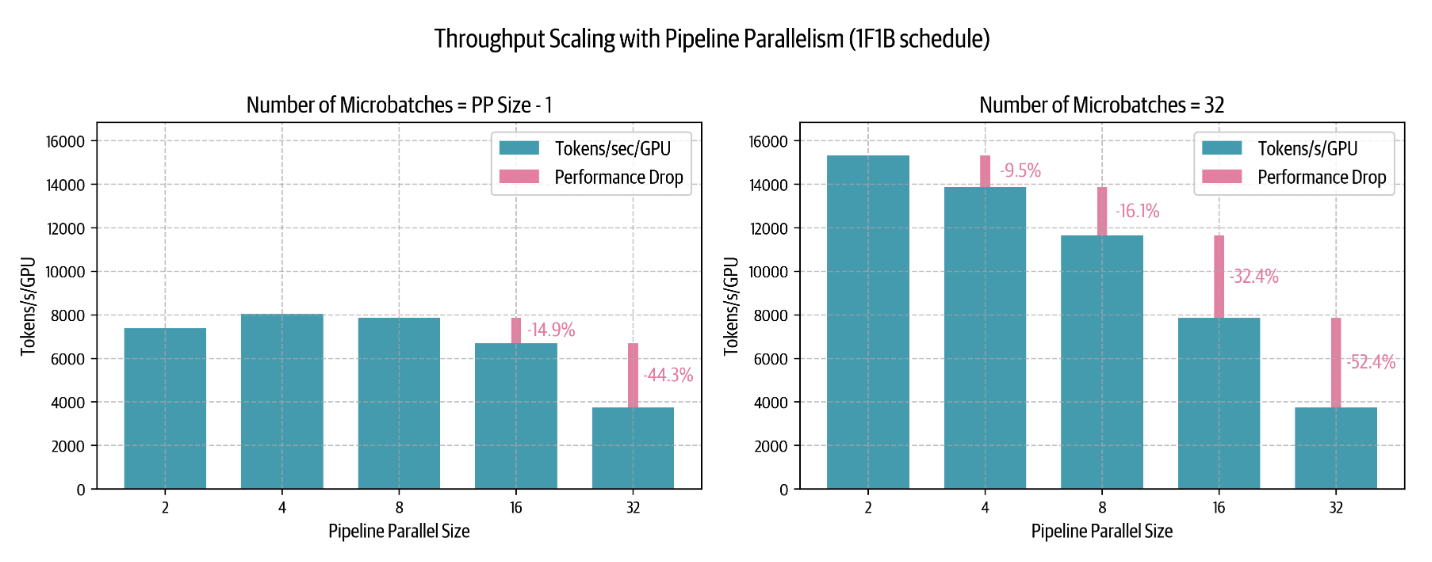
在图的左侧,当 micro-batch 的数量小于或等于流水线并行度减一(即 m = p − 1)时,我们可以看到“气泡”会带来多么严重的负面影响 —— 性能很低,甚至在扩大 PP 时还会进一步下降。图的右侧展示的是,当 micro-batch 数量远大于流水线并行度(比如m = 32 ≫ p - 1)时,在较小 PP 并行度下性能得到明显提升,尽管在非常大的 PP 并行度下仍然会受到限制。但在实际训练中,我们无法无限制地增加 micro-batch 数量以维持 m ≫ p − 1 的比率,最终一定会受限于一个固定的 全局 batch size。PP并行度(p)不论怎么增加,在 micro-batch 数量已经达到最大可能值的情况下,bubble还是按照r_bubble = (p − 1) / m 增长。
有趣的是,即使在 micro-batch 数量较少的情况下,将并行度从一个节点(p = 8)扩展到两个节点(p = 16)时,性能也只下降了 14%,这远好于张量并行(Tensor Parallelism)在类似跨节点场景中通常 43% 的性能下降。
- Pipeline 并行:只在 stage 之间传递一次激活;(PP中stage就是把model按层划分后的一部分连续层,每一段叫一个stage,每个stage分配给一个GPU或者一组GPU)
- Tensor 并行:每一层内部都要频繁通信,尤其在跨节点通信时受限于带宽;
所以流水线并行比张量并行更适合多节点训练(inter-node scaling)。虽然 1F1B 显著减少了激活值所占的显存,但是bubble仍然是主要效率瓶颈。由于气泡的大小仍与流水线阶段数成正比,我们仍然让宝贵的 GPU 算力处于空闲状态。所以诞生了:
3. Interleaving stages (IS)交错阶段
引入一些额外的通信操作来降低bubble大小
到目前为止,我们是按照模型的深度维度(model depth)以最简单的方式划分模型,比如把第 1–4 层放在第一个 GPU 上,第 5–8 层放在第二个 GPU 上。现在我们可以把奇数层(1, 3, 5, 7)放在第一个 GPU 上,偶数层(2, 4, 6, 8)放在第二个 GPU 上。
这样看起来像”looping pipeline”循环流水线,在forward计算的时候每个micro-batches会在GPU之间循环穿行。如下图:
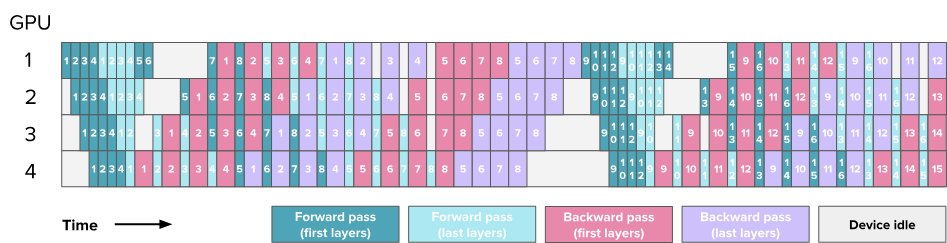
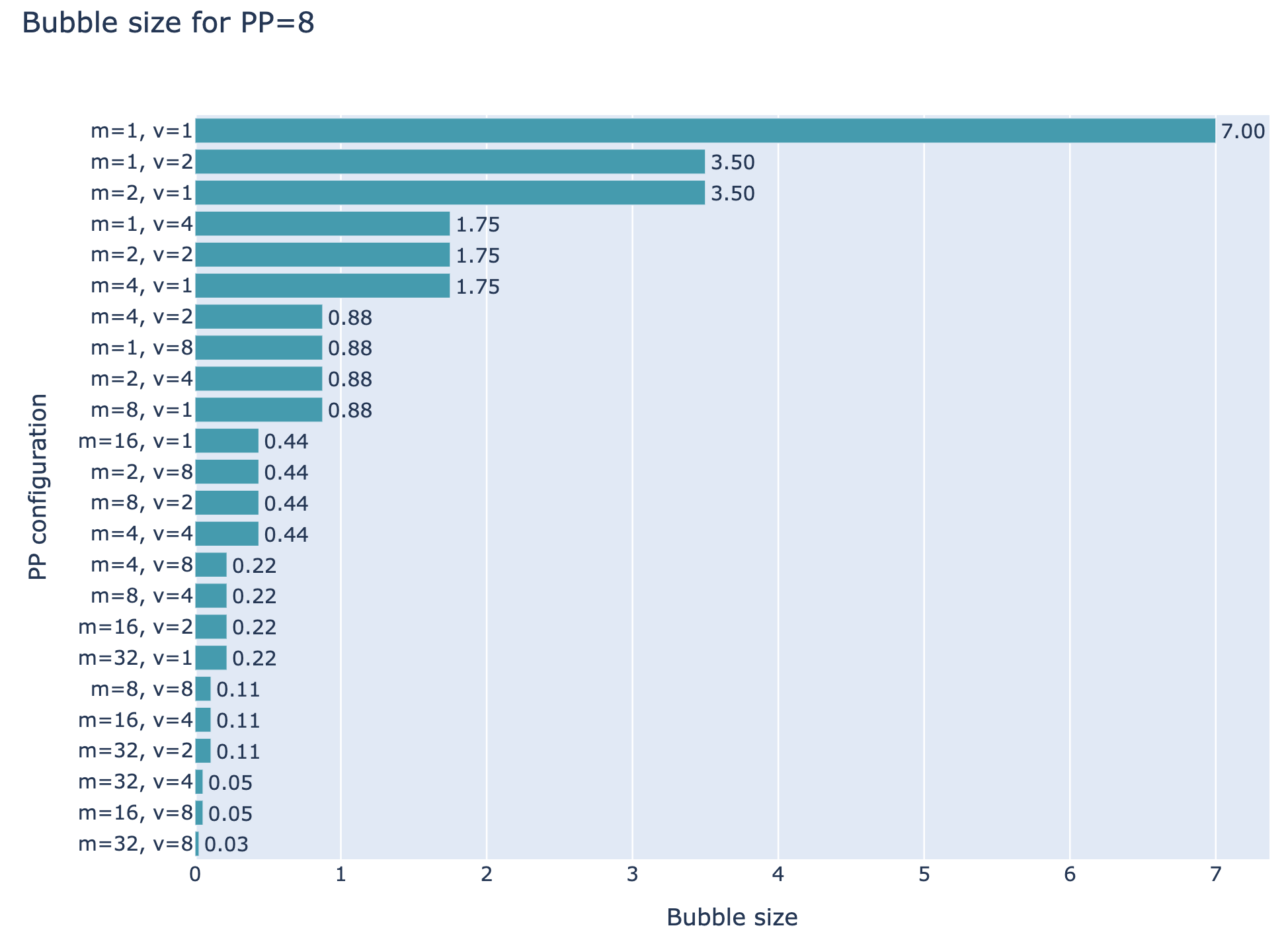
IS中需要额外的通信,因为同一段模型的计算,现在要多次经过每个 GPU,而在之前的方案中,仅需一次就能完成。现在每个Forward和Backward被除以一个因子 v,其中 v 是每个 GPU 上承载的 stage(或模型子块)的数量。这是因为我们能够更好地交错执行前向与反向传播。气泡时间和气泡占比公式如下:
关键性能提升的来源就是现在每个GPU不止运行一个stage,而是多个stage。pipeline中可并行计算粒度变小,流水线并密集。原本气泡的增长也会被v平均分摊。
因此,我们现在可以通过增加 micro-batches和使用交错阶段(v > 1)来减少 bubble。但需要注意的是,通信开销也会增加 v 倍,这是一种权衡。下图是并行度 p = 8 的流水线,然后增加m和v的情况:
调度会变复杂,每个GPU每个时刻需要做两种决策:
- 深度优先,尽快完成一个 batch 的整个前后传播
- 广度优先,尽可能填满整个流水线
选择的详细解释见论文:https://arxiv.org/pdf/2211.05953
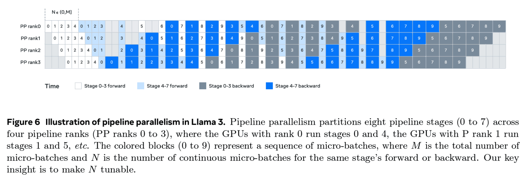
Llama 3.1 所采用的流水线并行策略所需的全部要素就是以上的部分,采用的是1F1B调度+IS交错阶段,并支持广度和深度优先之间调节。
接着,PP的新方法(DeepSeek方案https://arxiv.org/pdf/2412.19437)尝试将 bubble 几乎降为零;
4. Zero bubble and DualPipe
对涉及的计算操作进行更细粒度的划分,从而以**最有效的方式进行交错调度(interleaving)**这个的灵感是来源于Sea AI Lab 提出的 Zero Bubble 技术https://arxiv.org/pdf/2401.10241,促成了DualPipe。
在执行一个矩阵乘法的反向传播时,实际上涉及 两个独立的操作:
- 对输入的反向传播,记为 B;
- 对权重的反向传播,记为 W。
B(即对输入的反向传播)的输出是进行 下层的反向传播所必需的,而 W(即对权重的反向传播)不是立即必须的,通常只需在 执行优化器步骤(optimizer step)之前完成即可。